Using Deep Learning to Find Basketball Highlights

At Hudl, we would love to be able to watch every video uploaded to our servers and highlight the most impressive plays. Unfortunately, time constraints make this an impossible dream. There is, however, a group of people who have watched every game: the fans. Rather than polling these fans to find the best plays from every game, we decided to use their response to identify highlight-worthy plays.

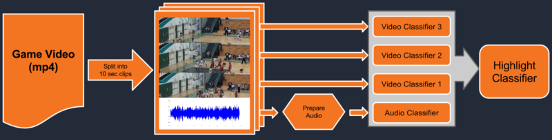
More specif­i­cal­ly, we will train classifiers that can recognize the difference between highlight worthy (signal) and non-highlight worthy (background) clips. The input to the classifiers will be the audio and video data and the output will be a score that represents the probability that the clip is highlight-worthy.

Training Sample

To select a sample of events to train our classifier on, we created a sample of 4153 clips, each 10 seconds long, from basketball games. No more than two clips come from the same basketball game and most are from different games played by different teams. This is to prevent the classifier from overfitting for a specific audience or arena. About half of these are clips during which a successful 3 point shot occurs. The other half are a semi-random selection of footage from basketball games.

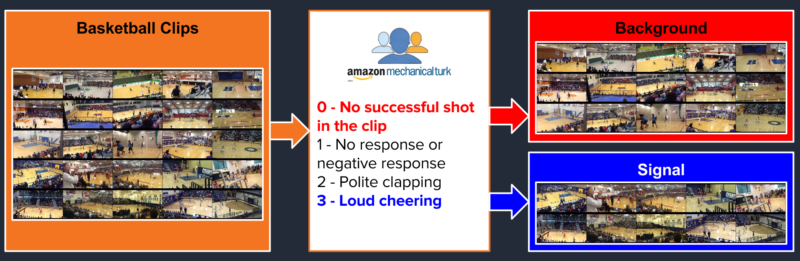
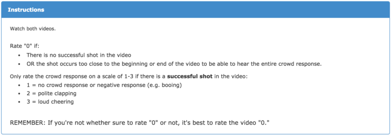
We used Amazon Mechanical Turk (mTurk) to separate the plays with the most cheering from those with no cheering or no successful shot. Each clip was sent to two or three separate Turkers. To separate highlight-worthy clips from non-highlight worthy clips, we gave two or three Turkers the following instructions:

The dis­tri­b­u­tion of average scores for the 4153 clips is shown below:

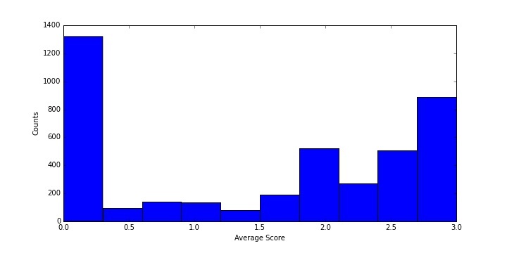
Clips that were unanimously scored as ​“3” were selected as our ​“cheering signal” while clips that were unanimously scored as ​“0” are considered to be background. This choice was made to provide maximum separation between signal and background. Moving forward, using a multi-class classifier that incor­po­rates clips with a ​“1” or a ​“2” could improve the performance of the classifier when it is used on entire games. For the time being, however, we use a sample of 887 signal clips and 1320 background clips.

Pre-Processing Audio

Before sending our audio data to a deep learning algorithm, we wanted to process it to make more intel­li­gi­ble than a series of raw audio amplitudes. We decided to convert our audio into an audio image that would reduce the data present in a 44,100 Hz wav file without losing the features that make it possible to distinguish cheering. To create an audio image, we went through the following steps:

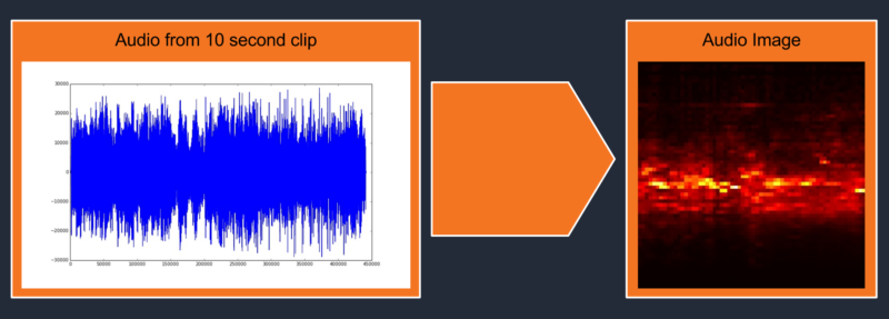
1. Convert the stereo audio to mono by dropping one of the two audio channels.
2. Use a fast Fourier transform to convert the audio from the time-domain to the frequency-domain.
3. Use 1/6 octave bands to slice the data into different frequency bins.
4. Convert each frequency bin back to the time-domain.
5. Create a 2D-map using the frequency bins as the Y-axis, the time as the X-axis and the amplitude as the Z-axis.

Video Classifiers

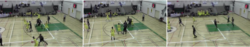
Although audio cheering seems like an obvious way to identify highlights, it is possible that the video could also be used to separate highlights. We decided to train three visual classifiers using raw frames from the video. The first classifier is trained on video frames taken from 2 second mark of each 10 second clip, the second is trained on frames taken from the 5 second mark of each clip, and the third is trained on frames taken from the 8 second mark of each clip. Below are shown rep­re­sen­ta­tive frames from an example clip at 2, 5, and 8 seconds (left to right).

Deep Learning Framework

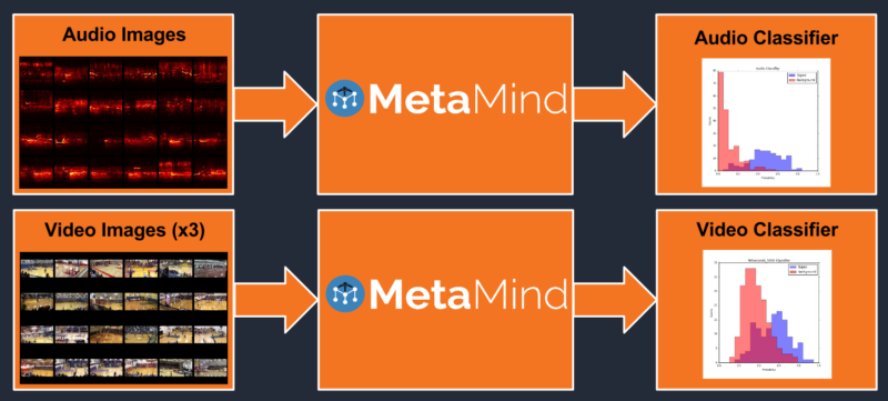
Because our 2D audio maps can be visualized as images, we decided to use Metamind as our deep learning engine. Metamind provides an easy-to-use Python API that lets the user train accurate image classifiers. Each classifier accepts as input an audio image and outputs a score that represents the probability that the prediction is correct.

Results

To train our classifier we split our 887 signal clips and 1320 background clips into train and test samples. 85% of the clips are used to train the classifiers while 15% of the clips are reserved to test the classifiers. In total, we trained four classifiers:

1. Audio Image
2. Video Frame (2 seconds)
3. Video Frame (5 seconds)
4. Video Frame (8 seconds)

Signal Background Separation

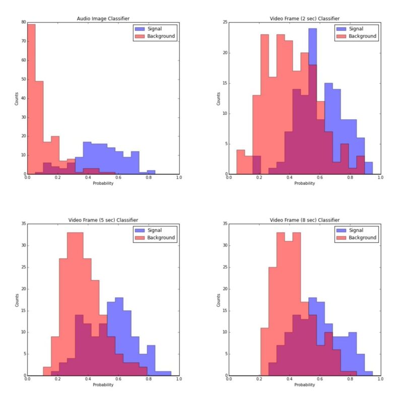
To test how well each classifier faired, we consider the predictions of the classifiers on the reserved test set. Because the classifier was not trained on these clips, overfitting cannot be causing the observed performance on the test set. The predictions for signal and background for each of the four classifiers are shown in the plots below. The X-axis is the predicted probability of being signal (i.e. the output variable of the classifier) and the Y-axis is the number of clips that were predicted to have that probability. The red histogram indicates background clips and the blue histogram indicates signal clips.

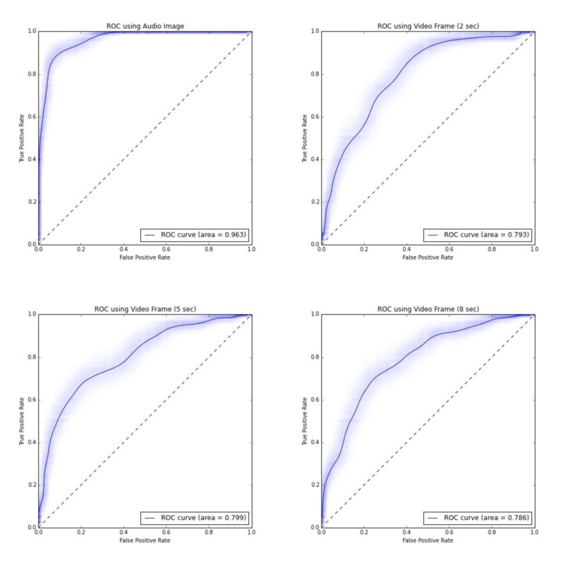
Receiver Operating Characteristic

The receiver operating char­ac­ter­is­tic (ROC) curve is a graphical way to illustrate the performance of a binary classifier when the dis­crim­i­na­tion threshold is changed. In our case, the dis­crim­i­na­tion threshold is the value of the output of our classifier above which a clip is determined to be signal. We can change this value to improve our true positive rate (the number of signal we correctly classify as signal) or reduce our false positive rate (the number of background that we incorrectly classify as signal). For example, by setting our threshold to 1, we would classify no clips as signal and thereby have 0% false positive rate (at the expense of a 0% true positive rate). Alternatively, we could set our threshold to 0 and classify all clips as signal thereby giving us a 100% true positive rate (at the expense of a 100% false positive rate).

The ROC curve for each of the four classifiers is shown below. A single number that represents the strength of a classifier is known as the ROC area under the curve (AUC). This integral represents how well a classifier is able to dif­fer­en­ti­ate between signal and background along all working points. The curves shown are the average of boot­strapped samples and the fuzzy band around the curve represent the possible ways in which the ROC curve could reasonably fluctuate.

Combining Classifiers

Because each of these classifiers provides different information, it’s possible that their combination could perform better than any single classifier alone. To combine classifiers we must train a third classifier that takes, as features, the prob­a­bil­i­ties from the original classifiers and returns a single probability.

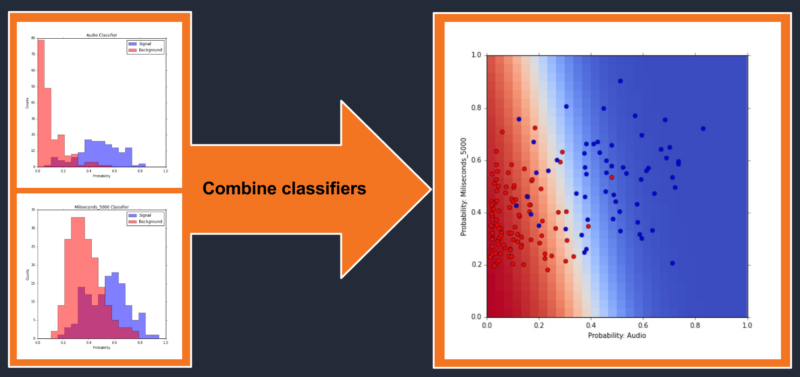
To visualize the performance of these combined classifiers we make a 2D plot with each axis rep­re­sent­ing the input probability. Each test clip is plotted as a point in this 2D-space and is colored blue, if signal, or red, if background. The prediction of the combined classifier is plotted in the background as a 2D-color map. The color represents the combined classifier’s predicted probability of being signal or background.

Combined Classifier Performance

We create the ROC curves as before in order to evaluate the performance of these combined classifiers. As expected, the combined classifiers which include the audio classifier perform the best and the improvement in ROC AUC from audio alone to audio plus video is 0.96 to 0.97. This is not a dramatic improvement, but it demon­strates that there are gains to be had from adding visual information. When two visual classifiers are added together, the ROC AUC increases from ~0.79 to ~0.83. This increase indicates that there is additional information to be gained from utilizing different times in the video.

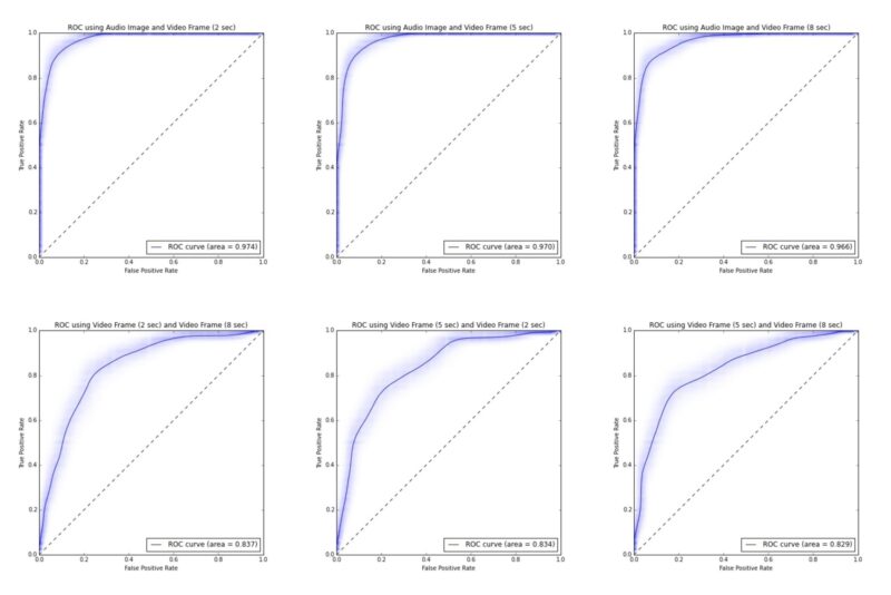
Final Combination

A final combination of all four classifiers was performed but this ultimate combination was no better than the pairwise combination of audio and video. This indicates that further improve­ments to our clas­si­fi­ca­tion would need to come from tweaks to the pre-processing of the data or the classifiers themselves rather than by simply adding additional video classifiers to the mix.

Full Game Testing

Despite the fact that we have evaluated our classifiers on test data, this testing has been performed in a very controlled setting. This is because the backgrounds we have used are not necessarily rep­re­sen­ta­tive of the clips present across an entire game. Furthermore, our ability to separate signal from background is useless if our top predictions in a specific game are not, in fact, among the top plays in that game.

To evaluate our classifier in the wild we will split four games into overlapping 10 second clips. Overlapping clips means that we make clips for 0 seconds to 10 seconds, 5 seconds to 15 seconds, 10 seconds to 20 seconds, etc… These clips are then passed through the audio classifier. Our goal in doing this this is to answer the following three questions:

1. What is the dis­tri­b­u­tion of prob­a­bil­i­ties for clips in a whole game?
2. How many of our ​“top picks” are highlight worthy?
3. Does our signal probability rating represent the true probability of a clip being signal?

Probability Distributions

The probability dis­tri­b­u­tion of clips for the four test games is found below.

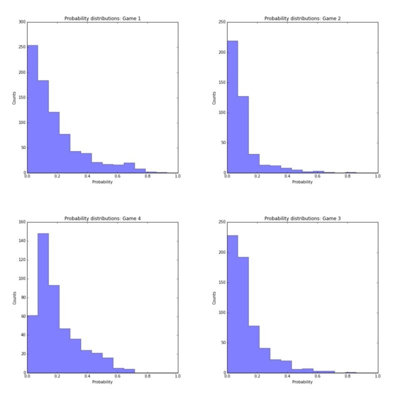
As is seen in the above images, the majority of clips are classified as background.

Top Picks

An animated gif for the top clip from each of the four test games is shown below. In addition, the top five clips from each game and their prob­a­bil­i­ties are shown and the content of each clip is discussed.

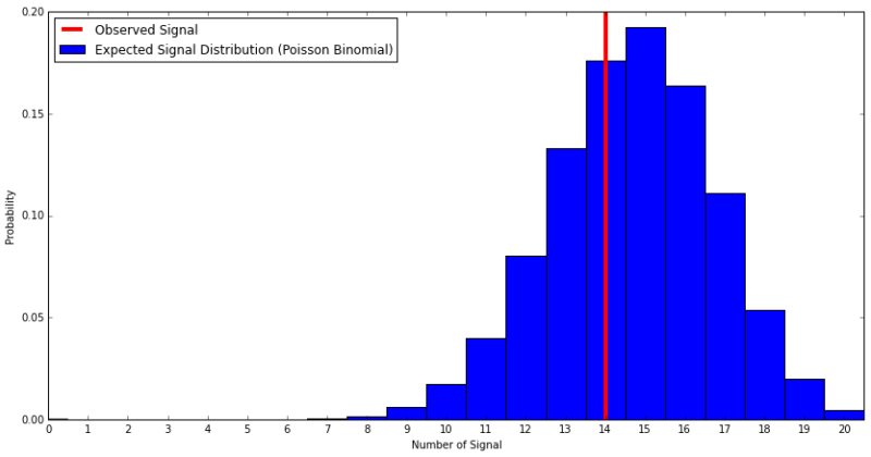
Of these, we would consider the made shots to be signal which gives us 14 signal out of 20 total clips. Additionally, the top play of each game is signal.

To understand our expec­ta­tions, we use the Poisson Binomial dis­tri­b­u­tion. The mean is the sum of all 20 prob­a­bil­i­ties and the standard deviation is the square root of the sum of probability*(1-probability) for each of the 20 prob­a­bil­i­ties. This indicates that we should expect 14.7 +/- 2.1 signal events. Our 14 observed signal events are consistent with this expectation as seen in the dis­tri­b­u­tion below.

Next Steps

There are many additional steps that could be used to improve the performance of the highlight classifier and there are a number of challenges to be solved before using the classifier is practical on a large scale.

Some of these are performance related: fast processing and creation of the audio images.

Others are more practical: we need to be able to determine which team a highlight is for so we don’t suggest that a player tag a highlight of them getting dunked on.

Additionally, there are improve­ments to the classifiers themselves: these can include an increase in the size of the training sample or performing more pre­pro­cess­ing of the data to make signal/​background dis­crim­i­na­tion easier.

The last and perhaps most important step is the opti­miza­tion of the video classifiers: right now these video classifiers provide minimal value when combined with the audio classifiers, but this value could be increased sub­stan­tial­ly if we were to standardize the location of the ​“cheering” within each clip. This would help us to distinguish between impressive successful shots, free throws, and plays that occur away from the basket.

It’s an exciting time for the product team at Hudl and we’re constantly coming up with innovative new projects to tackle. If you are interested in working with us to solve the next set of problems, check out our job postings!