The Low-Hanging Fruit of Redshift Performance

This post is part three of our blog series about Fulla, Hudl’s data warehouse. Part one talked about moving from Hive to Redshift and part two talked about loading in our application logging data. Part three was supposed to be about tailing the MongoDB oplog, but I decided to take a brief detour and tell you about some performance issues we started to run into after we hashed out our ETL cycle for logging data.

To begin, let’s rewind about a month. We had about 30 people using our Redshift cluster regularly, a few of whom were ​“power users” who used it constantly. Redshift was proving itself to be a great tool to learn about our users and how they use Hudl. However, with increased usage, bottlenecks became a lot more noticeable and increas­ing­ly painful to deal with. Queries that used to take 30 seconds were taking minutes. Some longer queries were taking more than an hour. While this might be reasonable for large analytical batch-jobs, it’s hardly acceptable for interactive querying.

We quickly learned that the biggest source of latency for us was our logs table. Some brief background on the logs table: it contains all of our application logs with common fields parsed out. Most of our application logs contain key-value pairs that look something like:

... Operation=View, Function=Highlight, App=Android, User=123456...

We parse out about 200 of the most common key-value pairs into their own special column in the logs table. I won’t go any further into how we populate the logs table since that’s already been covered in part two of this series. Instead I’m going to talk about some problems with the table.

Problems with the Logs Table

It’s a super useful table!
It contains information about how our users are actually using our products. Everyone wants to use it in almost every query. This is actually a really good problem to have. It means we’re providing people with something useful. However, it exacerbates some of our other problems.

It’s huge
It has more than 30 billion rows. This is a problem for several reasons. It requires queries to sift through much more data than they need to. It also makes it pro­hib­i­tive­ly slow to vacuum, which brings me to the next problem…

It was completely un-vacuumed
In Redshift, vacuuming does two things: 1) sorts the table based on a predefined sortkey and 2) reclaims unused disk space left after delete or update operations (here’s a good SO answer on why this is necessary). The logs table is generally only appended to, so we don’t really need to worry about reclaiming deleted space, however the sorting aspect is drastically important for us. The logs table had a sortkey, but the table was 0% sorted so most queries against the table had to do large table scans. We were also worried that it would take weeks to actually vacuum the table and would use all the cluster’s resources in the process.

None of the columns had encodings
This was problematic because it meant we weren’t using our disk space and memory efficiently. As a result the table took up 20 TB of our 32 TB cluster. In short, this means we couldn’t ever make a copy of the table to fix our problems.

It had a really wide column
We store the raw log message in a column alongside all the parsed out fields. If someone wanted a field from a log that we didn’t parse out, they had to extract it from the message field using regex or SQL wildcards. It was made even worse by the fact that the message column was of type VARCHAR(MAX) which means that 64K of memory had to be allocated for every single record that was read into memory. Even if the actual log message was only 1K, it still had to allocate 64K of memory for it. As a result all of the queries that touched the message field had to write to disk a lot when they ran out of memory. It was just… just awful.

Let’s Fix It!

As I mentioned above, our humble two-node Redshift cluster only has 32TB of space so there’s no way we could copy the 20 TB table within the same cluster. Additionally, we wanted to fix this problem without hindering performance and with minimal downtime since some people use it for their full-time job. With all that in mind, here’s the plan we came up with:

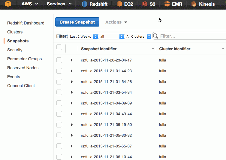
1. Spin up a new Redshift cluster from one of the snapshots that are taken regularly. The AWS Redshift console makes this super easy to do in about three clicks:

2. Drop the logs table on the new cluster. Re-create the table with messagetime as the sortkey and with the message column truncated to VARCHAR(1024). We chose VARCHAR(1024) because we realized >99% of the logs we were storing were shorter than that. What’s more, the logs that were longer were usually long stack traces which were typically not useful in the kind of offline analysis we use Fulla for.

3. Use the copy command to load in the most recent month’s logs into the table from S3. This will auto­mat­i­cal­ly set sensible column encodings for us.

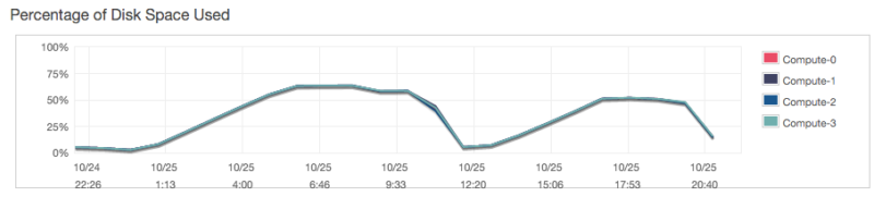
4. Use the copy command to load the rest of the logs from S3. This took about 18 hours total. It’s somewhat interesting how disk usage increases during a COPY and decreases afterwards (shown below). I assume this is because the files that were pulled from S3 get cleaned up after they’re loaded into the table.

5. Run vacuum logs;. This took about 4 days total. After we do all that, the new cluster is ready to use! We just need to switch over from the old cluster. Luckily, Redshift makes it possible to do this with minimal downtime and without needing to update the connection string on all of your clients! We renamed the old cluster from ​“fulla” to ​“fulla-old”, then renamed the new cluster from ​“fulla-new” to ​“fulla”. Overall, the switchover took about 10 minutes total and people were ready to start using the shiny new logs table.

After

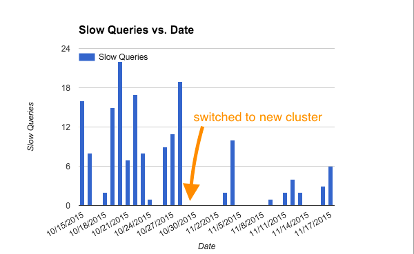
Some brief stats from after the migration. Between the column encodings, the truncated message column, and having the table vacuumed the total table size went from 20 TB to 5 TB. The number of ​“slow queries” we were detecting per day dropped sig­nif­i­cant­ly as can be seen in my fancy excel graph below:

During this time, overall usage has been steadily increasing as we’ve been educating more people on how to use Fulla:

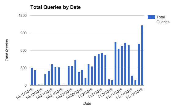
Despite this increase in usage, cluster performance has improved greatly!

Next Steps

Our improve­ments are not yet complete. The logs table is still the biggest bottleneck of working with our Redshift cluster. We’re putting a process in place to extract product-specific and team-specific tables from the log data rather than having everyone use one giant logolith (seewhatididthere.jpg). Another impending problem is that the logs table takes about 12 hours to vacuum. We kick off a vacuum job each night after we load in the logs from the previous day. To get that time down, we’re planning on breaking off logs from previous years and creating a view over multiple tables.

Main Takeaways

1. Vacuum your redshift tables. Vacuum early and vacuum often.
2. Make sure you have proper column encodings. The best way to do this is to let the copy command auto­mat­i­cal­ly set them for you if possible.
3. Avoid VARCHAR(MAX). When you have VARCHAR fields, be really con­ser­v­a­tive with their size. Don’t just default to VARCHAR(MAX) to avoid thinking about your data. There are real dis­ad­van­tages to having wide fields.

If you are working with Redshift and this article helped you, please let me know! We’re learning more about it every day and I’d love to swap tips and tricks with you. Stay tuned for part 4 of this series where I tell you all about tailing the MongoDB oplog.